Polarization of Light

Introduction:


This experiment explores the effects of polarizing filters angled with respect to one another on light intensity transmitted.  Selective absorption is the method of polarization for this activity.  Thus, perpendicularly angled filters should theoretically absorb all light that would pass through.  Parallel filters should transmit the most light.  Two filters will be used first and analyzed then three.

Steps:

Two Polarizing filter setup with light source shining through and lumens detector at end.

Example measurement at maximum transmission (theta = 0 degrees)

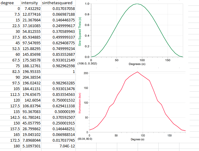
Data for two polarizers:

degree	intensity	costhetasquared
0	7.432292	0.017037058
7.5	12.07742	0.066987188
15	21.36766	0.146446375
22.5	37.16108	0.249999617
30	54.81256	0.370589943
37.5	85.93489	0.499999337
45	97.54769	0.629408775
52.5	125.883	0.749999234
60	145.857	0.853552687
67.5	175.5858	0.933012149
75	188.1276	0.982962598
82.5	196.9533	1
90	204.3855
97.5	196.0243	0.982963285
105	184.4115	0.933013476
112.5	174.6568	0.853554563
120	142.6054	0.750001532
127.5	106.8379	0.629411338
135	93.36708	0.50000199
142.5	61.78024	0.370592507
150	45.0578	0.250001915
157.5	28.79986	0.146448251
165	19.0451	0.066988514
172.5	7.896804	0.017037745
180	5.10973	7.04E-12

As expected, the plotted data is of cos^2 fit.

Three Polarizing filter:

Three polarizing filter setup.

Illumination vs cos^theta

In the three polarizing filter experiment, we notice that with the first and last filters at 90 degrees with respect to one another, the middle filter must be at 45 degrees to maximize transmission of light.


Conclusion:
Does the light from the fluorescent bulb have any polarization to it? If so, in what plane is the light polarized? How can you tell?

 No, the fluorescent bulb does not have any polarization associated with it.  You can tell this since a single polarizing filter cannot absorb a significant amount of light.  Two are needed.  One to first polarize the light, the other to absorb the polarized light transmitted through.

Does the reflected light have an polarization to it? If so, in what plane is the light polarized? How can you tell?

 Yes, the reflected light has polarization.  A filter may absorb an appreciable amount of the light once angled parallel to the table.

This lab does not lend itself to uncertainty calculations since our logger pro instrument was the only tool used here.  All values are averaged yet they exhibit the trends expected (light intensity if related to the cos^2 of the angle of the polarizing filter.  

CD Diffraction

Introduction:

Diffraction occurs in a multiple-slit experiment.  This experiment will explore the multiple grooves indented into a common compact disk.  The grooves on the disk will act as the multiple-slits in our diffraction experiment.  The spacing between the grooves will be obtained through the diffraction equation:

 and

where lambda is the wavelength of the laser used, m =1, y is the distance between first order maxima, and L is the distance between the screen of the laser diffraction pattern and the CD.


Steps:

First, we measure the wavelength of our laser.  To do this, we used a diffraction grating with 500 slits per millimeter and the equation mentioned above in a our calculations

Calculations for our laser wavelength are given below:

Since red light ranges around 700nm, we accept our calculations within our uncertainties provided.

After obtaining the wavelength parameter, we proceed to our CD diffraction apparatus seen below.

A parallel setup is accomplished by aligning the edges of our disk and cd placeholders along the edge of our table.  Clamps are aligned accordingly.  Diffraction patterns are marked on our paper screen and measured afterwards.

Calculating the distance between adjacent grooves is done in the calculations below

Questions/Conclusions:

The actual distance between the adjacent grooves on our compact disk is given by the manufacturer's standard value of 1.600 microns.  This gives us

The error is fairly large and falls well out of our uncertainty of .137 microns.
The nature of the experiment itself has multiple parameters and precision setups required.  Our results show  the same order of magnitude after uncertainty is taken into account.  So we are satisfied with this.  Another source of error might be the impurities of the compact disks we used.  This might account for a deviation from the manufacturer's standard value.

Measuring a Human Hair

Introduction:

The thickness of a human hair is about 50-150 micrometers.  In this experiment we will use interference patterns of light caused by a single human hair.  The hair acts as separator in a Young's double slit experiment and the thickness of it can be calculated as the d parameter in the equation

where y is the distance between adjacent interference maximas, lambda is the wavelength of the laser we will use, L is the distance between the hair and the screen of the patterns.

Steps:

The apparatus is depicted below:

For ease of measurement, a meter stick serves as the distance L.

Interference patterns observed (Previously marked patterns are shown above the laser lighting).

The distanced between markings were averaged after using calipers.

A micrometer is used as a means to compare our experimental data.

The results are tabulated below

Questions/Conclusions:

Using interference patterns to measure the diameter of the human hair is only so reliable.  We obtained a percent error of 9.2%, and were satisfied with the results since the interference equation involves many parameters that lead to greater uncertainty.  The micrometer has a sole purpose in measuring objects in these scales and so it was taken as the control in this experiment.

Lenses

Introduction:

Determining the focal length of a lens is a simple procedure that may be done by focusing parallel light rays that may be provided by the sun.  In this experiment, we will measure the focal length of thin converging lens and verify the relationship of the thin lens equation:


Steps:

The focal length is first found by measuring the actual distance from the lens the point of focus.  With limited sunlight on the day of this experiment, we were forced to improvise on our technique of measuring the focal length.  We used to lasers pointed into the lens.  The resulting intersection would be the focal point.

Improvised method of measuring converging lens focal length.

The measured focal length was

f = 5.0 ± 1.0 cm
The reason for our high uncertainty is that the intersection of the lasers was only apparent within a range of 1 cm. The experiment we ran varied the object distance at multiples of the focal length.
Object height is a constant as measured from the light box used.  Image distance and height were measured.

A screen is used for the projected image when the object distance is fairly small.

A ruler is used to measure image height at greater object distances.

The data collected is tabulated below.


d0 (± .1 cm) di (± .1 cm) h0 (± .1 cm) hi (± .1cm) M               
5f = 25.000         7.000           1.800         0.400 0.23 ± 0.07
4f = 20.000         7.300           1.800         0.600 0.34 ± 0.07
3f = 15.000         8.200           1.800         0.700 0.39 ± 0.08
2f = 10.000       10.500           1.800         1.800 1.0   ± 0.1
1.5f =7.500       18.700           1.800         4.100 2.3   ± 0.2



Calculating fmax and fmin from the given data we find
fmax = ( 1/(5f +.1) + 1/(7.0+.1) )^-1   = 5.53 cm
fmin  = ( 1/(2f -.1) + 1/(10.5-.1) )^-1   = 5.07 cm
At an object distance of .5f, the image is now virtual as seen behind the the lens.

A virtual image created by standing our object  ahead of our focal point

The lens equation describes an inverse relation ship between d0 and di.  We expect our di vs d0 to behave in this way.

Object distance vs Image distance (1)

Inverse Image Distance vs Negative Inverse Object Distance (2)

The characteristics of graph 2 are
Slope = .9475
y-intercept = .184


Questions/Conclusions:


Rearranging the thin lens equation we find

The focal length f is the constant y-intercept.  Our slope is approximately 1, as expected from the above equation. 

Equating 1/f = .184

the result is f = 5.43cm
This is the average taken from our experimental data.

The uncertainty cam be take to be (fmax-fmin)/2 = .2cm

f = 5.4 ± .2 cm

From our original measurement of f = 5.0 ± 1.0 cm, we are within uncertainty.

Thus, we obtain an error of 8.6% from our experimental measurements.

The table above shows that image distance and image height decrease as a function of object distance.  Our graphed data illustrated this as well.

Concave and Convex Mirrors

Introduction:

In this experiment we examine the images formed by convex and concave mirrors.  By way of direct observation and sample calculations, we will find the general behavior of such images formed.

Steps:

Convex Mirrors

In our physical observation of convex mirrors we found that objects placed at further distances would appear smaller than they really were.  This effect became less exaggerated as you come closer to the mirror (it seems to be more like the appropriate size).

When looking at the convex mirror at a distance, we note that the image looks further away than the object actually is.  I am holding up the camera phone (black sweater). Clearly, the cameras distance, relative to the mirror, is closer than imaged.

Calculations involving magnifications with a convex mirror:

Sample calculations for a convex mirror with actual measurements on the figure shown.

Concave Mirrors

Concave mirrors offered a much different perspective once viewed at distances greater than the focal length. Images were inverted and smaller than the objects really were.  Although the image was inverted, we still observed the same closer-to-the-real-size effect as we did with convex mirrors.  As we neared the concave mirror, though, there was a point where no clear image could be seen.  We note this to be the focal point.   The diagrams at the conclusion of this experiment will illustrate this phenomenon.

The inversion effect is clear in this photo of a concave mirror.  I (black sweater) observe the actual relative distance to be  closer than was imaged in the mirror.

Calculations involving magnifications with a concave mirror:

Sample calculations for a concavemirror with actual measurements on the figure shown.

Questions/Conclusions:

 The image descriptions can be summarized with ray diagrams of convex and concave mirrors shown below.

Convex mirror:

Sample ray diagram for convex mirrors.

Concave mirror:

Sample ray diagram for concave mirrors.

The inversion effect is clearly seen by they sketch above, but the diagrams below illustrate exactly when a right side up image may be observed.  It is clear an object at a focal point cannot focus for a concave mirror as the rays reflected come back parallel.

General behavior of a concave mirror found using 3 ray diagrams.

Introduction to Reflection and Refraction

Introduction: 

The nature of refraction and reflection angles may be explored with the aid of a semicircular acrylic glass piece.  In this experiment, we will explore the how light propagates through two different mediums. Namely, air and acrylic glass.  Air is approximated as vacuum with an index of refraction of 1.  Alerting our apparatus setup will allows to observe the critical angles of incidence.

Steps:

The apparatus requires the acrylic glass piece, a light box, a voltage generator, and a protractor.
Setup 1:
The light beam is aimed at the center of the flat side and exits through a radial path of the glass piece. Since we approximate air as vacuum it has the lower density of the two mediums.  The acrylic has the higher density.  Hence we go from low-high-low densities (once the lights exits back to air).

The setup for our first experimental run.  Angle of incidence is 0 degrees here.

Varying the angle of incidence by 5 degrees on each measurement we obtain the refraction angle along with their sin values.



θ1 θ2 sinθ1 sinθ2
0   0 0.000 0.000
5 3.5   0.087 0.061
10 5      0.174 0.087
15 9.3   0.259 0.162
20 12.6 0.342 0.218
25 16 0.423 0.276
30 17.5 0.500 0.301
35 22.2 0.574 0.378
40 25.5 0.643 0.431
45 28.5 0.707 0.477
50 31.5 0.766 0.522
55 35 0.819 0.574
60 37.5 0.866 0.609


Uncertainties (+/-)
uθ1 uθ2 usinθ1 usinθ2
1 1 0.017 0.017
1 1 0.017 0.017
1  1 0.017 0.017
1 1 0.017 0.017
1 1 0.016 0.017
1 1 0.016 0.017
1 1 0.015 0.017
1 1 0.014 0.016
1  1 0.013 0.016
1 1 0.012 0.015
1 1 0.011 0.015
1  1 0.010 0.014
1  1 0.009 0.014

We obtain the following graphs:

θ1 vs θ2

sinθ1 vs sinθ2

θ1 vs θ2 
mθ ≈ .64
sinθ1 vs sinθ2
msinθ ≈ .66

sinθ2/sinθ1 = .66

Setup 2:
The second setup involves using the curved surface of the semicircular acrylic.  Aiming the light beam at the curved surface and to the center of circle, we obtain straight beams passing through the piece.  This happens because the light beam is normal to the surface and thus creates a 0 degree angle of incidence.
The data obtained is shown below.

Curved surface incidence.

θ1 θ2 sinθ1 sinθ2
0 0 0.000 0.000
5 9.5 0.087 0.165
10 16.5 0.174 0.284
15 24.5 0.259 0.415
20 34 0.342 0.559
25 44 0.423 0.695
30 51.5 0.500 0.783
35 64.5 0.574 0.903
40 80    0.643 0.985


Uncertainties (+/-)
uθ1 uθ2 usinθ1 usinθ2
1 1 0.017 0.017
1 1 0.017 0.017
1         1 0.017 0.017
1 1 0.017 0.016
1 1 0.016 0.014
1 1 0.016 0.013
1         1 0.015 0.011
1 1 0.014 0.008
1         1 0.013 0.003


Similarly, we produce the following graphs:

θ1 vs θ2

sinθ1 vs sinθ2

θ1 vs θ2 
mθ ≈ 1.6 (ignoring 20 degree angle)
sinθ1 vs sinθ2
msinθ ≈ 1.5 


Questions/Conclusions:

We notice that beyond 40 degree we run into an issue when refraction no longer occurs and, instead, the light beam is completely reflected back inside the acrylic.

Using the axis variable we may fit have the equation:
sinθ2/sinθ1 = 1.5

This relationship is exactly inversely proportional to the equation obtained obtained in setup 1.  This is expected as the light beam, in setup 1, goes from low to high index of refraction mediums.  Setup 2 represents the opposite pathway.

The slope for setup 2 represents the refractive index.  The actual values for the refractive index of acrylic glass vary usually around a value of 1.49.

Electromagnetic Radiation

Introduction:
Antennas are known to transmit electromagnetic radiation and at measurable quantities when provided an alternating voltage source.  This principal behind this is the fact that Maxwell's equations state that a varying electric field (the voltage provided) induces magnetic field lines.  The combination of the two create propagating EM waves.   The voltage signal sent in this wave can be detected and measured.  This lab will explore voltage signal provided by a short antenna and measure the voltage as a function of distance from the detector, an oscilloscope. Assumptions and simplifications made will be discussed in the error/uncertainty analysis of the experiment.

Steps:

A BNC adapter will be used to receive the signal at the oscilloscope.
Simple tests are conducted to verify that the signal at our oscilloscope is generated by the antenna.

1)Check signal at short and far distances as the voltage should fall off as 1/r^3 closely and 1/r and greater distances
2) Vary the frequency at a reasonable distance to detect change in frequency at the oscilloscope.
3) Check close distance signal by varying angles of deflection to verify (sintheta)^2/r^2 voltage variations.

Signal will be minimized at close distance by varying angle of deflection.

Close distance signals fall off as 1/r^3

Data is collected by varying distance from the adapter (measured around its base).

A meter stick is used to approximate 5cm increments.  Signal strength decreases as a function of distance.

Peak to Peak Voltages(Y axis -Volts) as a function of distance(X axis - meters)

A/r fit

A/r^3 fit

A/r^n fit (n=.6)

As we observe, the plotted data fits a more A/r fit.  As long term data collection shows, voltage falls off mostly as A/r.
In this case, are A/r^n resulted in n =.6
The results may differ here because we do no vary at great enough distances to really obtain the A/r relationship of distance and voltage.

Theoretically our voltage may be derived to be



Where L is the length of the antenna, z is the distance from the adapter, and the charge Q is calculated from experimental data.



Distnace (m) Vtheoretical P2P
0
0.05                 0.011631
0.1                   0.005687
0.15                 0.003616
0.2                   0.002704
0.25                 0.002234
0.3                   0.001965
0.35           0.001796

The theoretical peak to peak voltage plot is shown below:

Theoretical peak to peak voltage (V) vs distance (m)

Comparing the graphs above to our theoretical peak to peak voltage, it is clear that experimental data and theoretical agree on the inverse relationship of voltage sensed as a function of distance (z).  Experimental results are not smooth and continuous as theoretical results.  This is caused by the inconsistencies in the inverse power relationship among distance and voltage—experimentally, we will experience a 1/r^3 relationship at close distances and tend towards 1/r at large enough distances.

Measurement Uncertainty:

Peak to Peak Voltage
ΔV = ±1mV

Quantization uncertainty for z:
Δz = ±.01m

accounting for BNC adapter length:
Δz = ±.05m







Questions/Conclusions:

Comparing our experimental results to theoretical we see that there is plenty of room for error given the above equations.  If we compare our theoretical values with experimental, our results agree within the same orders of magnitudes(mostly).
In our model we made several simplifications. We assumed linear charge density. Also, we did not take into account any interference from nearby wires and lab equipment.  We ignored fringing effects of the antenna rod that lead to different electric field distributions.
Future experiments may actually measure current supplied by our voltage generator to improve charge calculations.  Although negligible,  our calculations may also include the energy lost due resistance in the copper antenna.