Standing Waves

Introduction:
 Waves on a string are useful in the study of standing waves.  Given a well-controlled apparatus setup, we may look at the properties of such waves.  This experiment will study the number of nodes present, wavelength, frequency, and wave speed of waves after creating 10 harmonics for each of two case setups.

Steps:

The apparatus is depicted in the following two images:

A mass-pulley system is set up on one end of the string to create the tension needed .

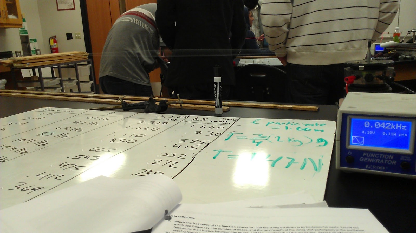Below the standing wave, meter sticks are aligned to measure distance between nodes and find wavelength. A frequency generator and wave driver attached to the string will produce oscillations necessary to obtain empirical data.

In the two cases studied data was collected by adjusting our frequency to create the first 10 harmonics.  Case 1 and Case two had different masses attached to vary the frequency.  The mass of the string was

mstring = .72 +/- .01g
lstring = 2.26 +/- .01m

μstring = mstring/lstring =   .319 +/- .006 g/m

CASE 1:
m1 = .200 +/- .001kg
T1 = 1.96 +/- .01N


CASE 2:
m2 = .050 +/- .001kg
T2 = .49 +/- .01N

CASE 1:

Harmonic n	frequency +/- 1Hz	fn = nf1 +/- n1Hz	λ  +/- .01m	Δx nodes +/- .005m
1	24	24	3.32	1.66
2	48	48	1.66	0.83
3	72	72	1.11	0.555
4	96	96	0.83	0.425
5	120	120	0.66	0.33
6	144	144	0.55	0.275
7	169	168	0.465	0.233
8	193	192	0.405	0.203
9	217	216	0.365	0.183
10	241	240	0.33	0.165

 CASE 2:

Harmonic n	frequency +/- 1Hz	fn = nf1 +/- n1Hz	λ  +/- .01m	Δx nodes +/- .005m
1	12	12	3.32	1.66
2	24	24	1.66	0.83
3	36	36	1.11	0.555
4	48	38	0.83	0.415
5	60	60	0.663	0.332
6	72	72	0.543	0.272
7	84	84	0.475	0.238
8	96	96	0.412	0.206
9	109	108	0.369	0.185
10	121	120	0.334	0.167

Plotting frequency vs 1/λ we obtain the following charts

Two equations may be used for calculation of speed of the wave, they are given by

and

The latter equation is seen by the slope of the plots above.
For theoretical calculations we may use our tension/density equation and obtain:


v1 = 78.4 +/- .9 m/s

v2 = 39.2 +/- .8 m/s

Questions/Conclusion:
The data table above shows the wavelength and the n values that describe the wave ( the harmonic).  It is clear that the wavelength follows the equation:

The plots of frequency versus 1/λ compare nicely with our theoretical wave speed obtained and fall within uncertainty of the results.  The sources of error associated with the variables required (T, μstring, λ, and f) are all instrumental and amounted to relatively small uncertainty as seen by the final result of our theoretical wavespeeds v1 and v2 .  Taking the percent error we find:
|v1 - slope1|/v1 * 100% = .60%
|v2 - slope2|/v2 * 100% = 2.1%

The ratio of the the predicted wave speed was
v1/v2 = 78.4/39.2 = 2.0
or we could use

Comparing this to our slope1 and slope2
slope1/slope2 = 78.867/40.02 = 1.97
A percent error of 1.5% on this ratio shows much agreement between the ratios

As seen by the the charts above our values for nf1 agree identically up until the last four frequency values for case 1 and up until the last 2 values for case 2.  Each disagreement is from these last couple of values is only +/- 1 Hz which is within the uncertainty provided (The smallest denomination on our frequency generator was 1Hz and so this was taken as the uncertainty value).

Taking a ratio of our frequencies from case 1 and case 2 we obtain

Harmonic	f1/f2
1	2
2	2
3	2
4	2
5	2

The obvious pattern is that the ratio is 2.  This makes sense since the velocity increased by a factor of 2 and the wavelengths for the corresponding harmonics were kept relatively constant.